Continuous Probability
A Brief Introduction to Continuous Probability
Up to now we have focused exclusively on discrete probability spaces \(\Omega\), where the number of sample points \(\omega\in\Omega\) is either finite or countably infinite (such as the integers). As a consequence, we have only been able to talk about discrete random variables, which take on only a finite or countably infinite number of values.
But in real life many quantities that we wish to model probabilistically are real-valued; examples include the position of a particle in a box, the time at which an certain incident happens, or the direction of travel of a meteorite. In this lecture, we discuss how to extend the concepts we’ve seen in the discrete setting to this continuous setting. As we shall see, everything translates in a natural way once we have set up the right framework. The framework involves some elementary calculus but (at this level of discussion) nothing too scary.
Continuous Uniform Probability Space
Suppose we spin a “wheel of fortune" and record the position of the pointer on the outer circumference of the wheel. Assuming that the circumference is of length \(\ell\) and that the wheel is unbiased, the position is presumably equally likely to take on any value in the real interval \([0,\ell]\). How do we model this experiment using a probability space?
Consider for a moment the analogous discrete setting, where the pointer can stop only at a finite number \(m\) of positions distributed evenly around the wheel. (If \(m\) is very large, then this is in some sense similar to the continuous setting, which we can think of as the limit \(m \to \infty\).) Then we would model this situation using the discrete sample space \(\Omega = \{0,\ell/m,2\ell/m,\dotsc,(m-1)\ell/m\}\), with uniform probabilities \({\mathbb{P}}[\omega] = 1/m\) for each \(\omega\in\Omega\).
In the continuous setting, however, we get into trouble if we try the same approach. If we let \(\omega\) range over all real numbers in \(\Omega = [0,\ell]\), what value should we assign to each \({\mathbb{P}}[\omega]\)? By uniformity, this probability should be the same for all \(\omega\). But if we assign \({\mathbb{P}}[\omega]\) to be any positive value, then because there are infinitely many \(\omega\) in \(\Omega\), the sum of all probabilities \({\mathbb{P}}[\omega]\) will be \(\infty\)! Thus, \({\mathbb{P}}[\omega]\) must be zero for all \(\omega\in\Omega\). But if all of our sample points have probability zero, then we are unable to assign meaningful probabilities to any events!
To resolve this problem, consider instead any non-empty interval \([a,b]\subseteq[0,\ell]\). Can we assign a non-zero probability value to this interval? Since the total probability assigned to \([0,\ell]\) must be \(1\), and since we want our probability to be uniform, the logical value for the probability of interval \([a,b]\) is \[\frac{\text{length of $[a,b]$}}{\text{length of $[0,\ell]$}} = \frac{b-a}{\ell}.\] In other words, the probability of an interval is proportional to its length.
Note that intervals are subsets of the sample space \(\Omega\) and are therefore events. So in contrast to discrete probability, where we assigned probabilities to points in the sample space, in continuous probability we are assigning probabilities to certain basic events (in this case intervals). What about probabilities of other events? By specifying the probability of intervals, we have also specified the probability of any event \(E\) which can be written as the disjoint union of (a finite or countably infinite number of) intervals, \(E=\bigcup_i E_i\). For then we can write \({\mathbb{P}}[E] = \sum_i {\mathbb{P}}[E_i]\), in analogous fashion to the discrete case. Thus for example the probability that the pointer ends up in the first or third quadrants of the wheel is \[\frac{\ell/4}{\ell}+\frac{\ell/4}{\ell} = \frac{1}{2}.\] For all practical purposes, such events are all we really need.1
Continuous Random Variables
Recall that in the discrete setting we typically work with random variables and their distributions, rather than directly with probability spaces and events. The simplest example of a continuous random variable is the position \(X\) of the pointer in the wheel of fortune, as discussed above. This random variable has the uniform distribution on \([0,\ell]\). How, precisely, should we define the distribution of a continuous random variable? In the discrete case the distribution of a r.v. \(X\) is described by specifying, for each possible value \(a\), the probability \({\mathbb{P}}[X=a]\). But for the r.v. \(X\) corresponding to the position of the pointer, we have \({\mathbb{P}}[X=a]=0\) for every \(a\), so we run into the same problem as we encountered above in defining the probability space.
The resolution is the same: instead of specifying \({\mathbb{P}}[X=a]\), we specify \({\mathbb{P}}[a\le X\le b]\) for all intervals \([a,b]\).2 To do this formally, we need to introduce the concept of a probability density function (sometimes referred to just as a “density", or a “pdf").
Definition 1 (Density)
A probability density function for a real-valued random variable \(X\) is a function \(f:{\mathbb{R}}\to{\mathbb{R}}\) satisfying:
\(f\) is non-negative: \(f(x) \ge 0\) for all \(x \in {\mathbb{R}}\).
The total integral of \(f\) is equal to \(1\): \(\int_{-\infty}^\infty f(x) \, {\mathrm{d}}x = 1\).
Then the distribution of \(X\) is given by: \[{\mathbb{P}}[a\le X\le b] = \int_{a}^b f(x) \, {\mathrm{d}}x\qquad\text{for all $a\le b$}.\]
Let’s examine this definition. Note that the definite integral is just the area under the curve \(f\) between the values \(a\) and \(b\). Thus \(f\) plays a similar role to the “histogram" we sometimes draw to picture the distribution of a discrete random variable. The first condition that \(f\) be non-negative ensures that the probability of every event is non-negative. The second condition that the total integral of \(f\) equal to \(1\) ensures that it defines a valid probability distribution, because the r.v. \(X\) must take on real values: \[ {\mathbb{P}}[X \in {\mathbb{R}}] = {\mathbb{P}}[-\infty < X < \infty] = \int_{-\infty}^\infty f(x) \, {\mathrm{d}}x = 1.\](1)
For example, consider the wheel-of-fortune r.v. \(X\), which has uniform distribution on the interval \([0,\ell]\). This means the density \(f\) of \(X\) vanishes outside this interval: \(f(x)=0\) for \(x<0\) and for \(x>\ell\). Within the interval \([0,\ell]\) we want the distribution of \(X\) to be uniform, which means we should take \(f\) to be a constant \(f(x)=c\) for \(0\le x\le\ell\). The value of \(c\) is determined by the requirement Equation 1 that the total area under \(f\) is \(1\): \[1 = \int_{-\infty}^\infty f(x) \, {\mathrm{d}}x = \int_{0}^\ell c \, {\mathrm{d}}x = c\ell,\] which gives us \(c=1/\ell\). Therefore, the density of the uniform distribution on \([0,\ell]\) is given by \[f(x) = \begin{cases} 0 & \text{for $x<0$;}\cr 1/\ell & \text{for $0\le x\le\ell$;}\cr 0 & \text{for $x>\ell$.}\cr \end{cases}\]
Remark:
Following the “histogram" analogy above, it is tempting to think of \(f(x)\) as a “probability". However, \(f(x)\) doesn’t itself correspond to the probability of anything! In particular, *there is no requirement that \(f(x)\) be bounded above by \(1\). For example, the density of the uniform distribution on the interval \([0,\ell]\) with \(\ell = 1/2\) is equal to \(f(x) = 1/(1/2) = 2\) for \(0 \le x \le 1/2\), which is greater than \(1\). To connect density \(f(x)\) with probabilities, we need to look at a very small interval \([x,x+\delta]\) close to \(x\); then we have \[ {\mathbb{P}}[x\le X\le x+\delta] = \int_{x}^{x+\delta} f(z) \, {\mathrm{d}}z \approx \delta f(x).\](2) Thus, we can interpret \(f(x)\) as the “probability per unit length" in the vicinity of \(x\).
Expectation and Variance
As in the discrete case, we define the expectation of a continuous r.v. as follows:
Definition 2 (Expectation)
The expectation of a continuous r.v. \(X\) with probability density function \(f\) is \[{\mathbb{E}}[X] = \int_{-\infty}^\infty xf(x) \, {\mathrm{d}}x.\]
Note that the integral plays the role of the summation in the discrete formula \({\mathbb{E}}[X] = \sum_a a{\mathbb{P}}[X=a]\). Similarly, we can define the variance as follows:
Definition 3 (Variance)
The variance of a continuous r.v. \(X\) with probability density function \(f\) is \[{\operatorname{var}}(X) = {\mathbb{E}}[(X-{\mathbb{E}}[X])^2] = {\mathbb{E}}[X^2] - {\mathbb{E}}[X]^2 = \int_{-\infty}^\infty x^2 f(x) \, {\mathrm{d}}x \;- \left(\int_{-\infty}^\infty xf(x) \, {\mathrm{d}}x\right)^2.\]
Example: Let \(X\) be a uniform r.v. on the interval \([0,\ell]\). Then intuitively, its expected value should be in the middle, \(\ell/2\). Indeed, we can use our definition above to compute \[{\mathbb{E}}[X] = \int_{0}^\ell x\frac{1}{\ell} \, {\mathrm{d}}x = \left[\frac{x^2}{2\ell}\right]_0^\ell = \frac{\ell}{2},\] as claimed. We can also calculate its variance using the above definition and plugging in the value \({\mathbb{E}}[X] = \ell/2\) to get: \[{\operatorname{var}}(X) = \int_{0}^\ell x^2\frac{1}{\ell} \, {\mathrm{d}}x - {\mathbb{E}}[X]^2 = \left[\frac{x^3}{3\ell}\right]_0^\ell - \left(\frac{\ell}{2}\right)^2 = \frac{\ell^2}{3} - \frac{\ell^2}{4} = \frac{\ell^2}{12}.\] The factor of \(1/12\) here is not particularly intuitive, but the fact that the variance is proportional to \(\ell^2\) should come as no surprise. Like its discrete counterpart, this distribution has large variance.
Joint Distribution
Recall that for discrete random variables \(X\) and \(Y\), their joint distribution is specified by the probabilities \({\mathbb{P}}[X = a, Y = c]\) for all possible values \(a,c\). Similarly, if \(X\) and \(Y\) are continuous random variables, then their joint distributions are specified by the probabilities \({\mathbb{P}}[a \le X \le b, c \le Y \le d]\) for all \(a \le b\), \(c \le d\). Moreover, just as the distribution of \(X\) can be characterized by its density function, the joint distribution of \(X\) and \(Y\) can be characterized by their joint density.
Definition 4 (Joint Density)
A joint density function for two random variable \(X\) and \(Y\) is a function \(f:{\mathbb{R}}^2\to{\mathbb{R}}\) satisfying:
\(f\) is non-negative: \(f(x,y) \ge 0\) for all \(x,y \in {\mathbb{R}}\).
The total integral of \(f\) is equal to \(1\): \(\int_{-\infty}^\infty \int_{-\infty}^\infty f(x,y) \, {\mathrm{d}}x \, {\mathrm{d}}y = 1\).
Then the joint distribution of \(X\) and \(Y\) is given by: \[{\mathbb{P}}[a\le X\le b, ~ c \le Y \le d] = \int_{c}^d \int_a^b f(x,y) \, {\mathrm{d}}x \, {\mathrm{d}}y\qquad\text{for all $a\le b$ and $c \le d$}.\]
In analogy with Equation 2, we can connect the joint density \(f(x,y)\) with probabilities by looking at a very small square \([x,x+\delta] \times [y,y+\delta]\) close to \((x,y)\); then we have \[ {\mathbb{P}}[x\le X\le x+\delta, ~ y \le Y \le y +\delta] = \int_y^{y+\delta}\int_{x}^{x+\delta} f(u,v) \, {\mathrm{d}}u \, {\mathrm{d}}v \approx \delta^2 f(x,y).\](3) Thus we can interpret \(f(x,y)\) as the “probability per unit area" in the vicinity of \((x,y)\).
Independence
Recall that two discrete random variables \(X\) and \(Y\) are said to be independent if the events \(X=a\) and \(Y=c\) are independent for every possible values \(a,c\). We have a similar definition for continuous random variables:
Definition 5 (Independence for Continuous R.V.s)
Two continuous r.v.’s \(X,Y\) are independent if the events \(a\le X\le b\) and \(c\le Y\le d\) are independent for all \(a \le b\) and \(c \le d\): \[{\mathbb{P}}[a \le X \le b, ~ c \le Y \le d] = {\mathbb{P}}[a \le X \le b] \cdot {\mathbb{P}}[c \le Y \le d].\]
What does this definition say about the joint density of independent r.v.’s \(X\) and \(Y\)? Applying Equation 3 to connect the joint density with probabilities, we get, for small \(\delta\): \[\begin{aligned} \delta^2 f(x,y) & \approx {\mathbb{P}}[x\le X\le x+\delta, ~ y \le Y \le y +\delta]\\ & = {\mathbb{P}}[x\le X\le x+\delta] \cdot {\mathbb{P}}[y \le Y \le y +\delta]\qquad\text{(by independence)}\\ & \approx \delta f_X(x) \times \delta f_Y(y) \\ &= \delta^2 f_X(x) f_Y(y),\end{aligned}\] where \(f_X\) and \(f_Y\) are the (marginal) densities of \(X\) and \(Y\) respectively. So we get the following result:
Theorem 1
The joint density of independent r.v.’s \(X\) and \(Y\) is the product of the marginal densities: \[f(x,y) = f_X(x) \, f_Y(y) ~~ \text{ for all } ~ x,y \in {\mathbb{R}}.\]
Two Important Continuous Distributions
We have already seen one important continuous distribution, namely the uniform distribution. In this section we will see two more: the exponential distribution and the normal (or Gaussian) distribution. These three distributions cover the vast majority of continuous random variables arising in applications.
Exponential Distribution
The exponential distribution is a continuous version of the geometric distribution, which we have already seen in the previous note. Recall that the geometric distribution describes the number of tosses of a coin until the first Head appears; the distribution has a single parameter \(p\), which is the bias (Heads probability) of the coin. Of course, in real life applications we are usually not waiting for a coin to come up Heads but rather waiting for a system to fail, a clock to ring, an experiment to succeed, etc.
In such applications we are frequently not dealing with discrete events or discrete time, but rather with continuous time: for example, if we are waiting for an apple to fall off a tree, it can do so at any time at all, not necessarily on the tick of a discrete clock. This situation is naturally modeled by the exponential distribution, defined as follows:
Definition 6 (Exponential Distribution)
For \(\lambda>0\), a continuous random variable \(X\) with density function \[f(x) = \begin{cases} \lambda e^{-\lambda x} & \text{if $x\ge 0$};\\ 0 & \text{otherwise}. \end{cases}\] is called an exponential random variable with parameter \(\lambda\).
Note that by definition \(f(x)\) is non-negative. Moreover, we can check that it satisfies Equation 1: \[\int_{-\infty}^\infty f(x) \, {\mathrm{d}}x = \int_0^\infty \lambda e^{-\lambda x} \, {\mathrm{d}}x = \bigl[-e^{-\lambda x}\bigr]_0^\infty = 1,\] so \(f(x)\) is indeed a valid probability density function. Figure 1 shows the plot of the density function for the exponential distribution with \(\lambda = 2\).
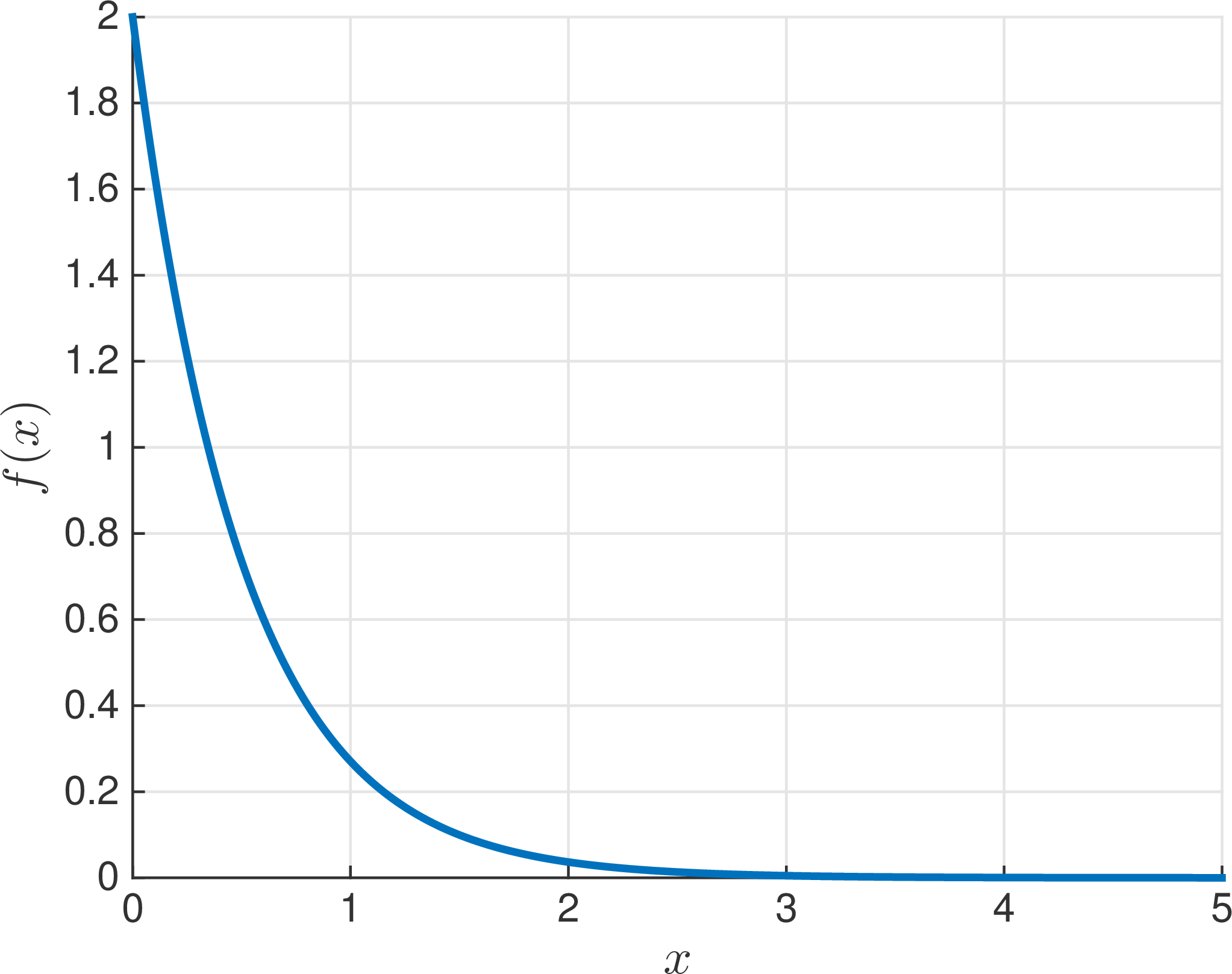
Figure 1: The density function for the exponential distribution with \(\lambda = 2\).
Let us now compute its expectation and variance.
Theorem 2
Let \(X\) be an exponential random variable with parameter \(\lambda > 0\). Then \[{\mathbb{E}}[X] = \frac{1}{\lambda} \qquad \text{ and } \qquad {\operatorname{var}}(X) = \frac{1}{\lambda^2}.\]
Proof. We can calculate the expected value using integration by parts: \[{\mathbb{E}}[X] = \int_{-\infty}^\infty xf(x) \, {\mathrm{d}}x = \int_0^\infty \lambda xe^{-\lambda x} \, {\mathrm{d}}x = \bigl[-xe^{-\lambda x}\bigr]_0^\infty + \int_0^\infty e^{-\lambda x} \, {\mathrm{d}}x = 0 + \left[-\frac{e^{-\lambda x}}{\lambda}\right]_0^\infty = \frac{1}{\lambda}.\] To compute the variance, we first evaluate \({\mathbb{E}}[X^2]\), again using integration by parts: \[{\mathbb{E}}[X^2] = \int_{-\infty}^\infty x^2f(x) \, {\mathrm{d}}x = \int_0^\infty \lambda x^2e^{-\lambda x} \, {\mathrm{d}}x = \bigl[-x^2e^{-\lambda x}\bigr]_0^\infty + \int_0^\infty 2xe^{-\lambda x} \, {\mathrm{d}}x = 0 + \frac{2}{\lambda}{\mathbb{E}}[X] = \frac{2}{\lambda^2}.\] The variance is therefore \[{\operatorname{var}}(X) = {\mathbb{E}}[X^2] - {\mathbb{E}}[X]^2 = \frac{2}{\lambda^2} - \frac{1}{\lambda^2} = \frac{1}{\lambda^2},\] as claimed. \(\square\)
Exponential Distribution is the Continuous-Time Analog of Geometric Distribution
Like the geometric distribution, the exponential distribution has a single parameter \(\lambda\), which characterizes the rate at which events happen. Note that the exponential distribution satisfies, for any \(t\ge 0\), \[ {\mathbb{P}}[X> t] = \int_t^\infty \lambda e^{-\lambda x} \, {\mathrm{d}}x = \bigl[-e^{-\lambda x}\bigr]_t^\infty = e^{-\lambda t}.\](4) In other words, the probability that we have to wait more than time \(t\) for our event to happen is \(e^{-\lambda t}\), which is an exponential decay with rate \(\lambda\).
Now consider a discrete-time setting in which we perform one trial every \(\delta\) seconds (where \(\delta\) is very small — in fact, we will take \(\delta\to 0\) to make time “continuous"), and where our success probability is \(p=\lambda\delta\). Making the success probability proportional to \(\delta\) makes sense, as it corresponds to the natural assumption that there is a fixed rate of success per unit time, which we denote by \(\lambda = p/\delta\). In this discrete setting, the number of trials until we get a success has the geometric distribution with parameter \(p\), so if we let the r.v. \(Y\) denote the time (in seconds) until we get a success we have \[{\mathbb{P}}[Y> k\delta] = (1-p)^k = (1-\lambda\delta)^k \qquad\text{for any $k\ge 0$}.\] Hence, for any \(t>0\), we have \[ {\mathbb{P}}[Y> t] = {\mathbb{P}}\!\left[Y>\left(\frac{t}{\delta}\right)\delta\right] = (1-\lambda\delta)^{t/\delta} \approx e^{-\lambda t},\](5) where this final approximation holds in the limit as \(\delta\to 0\) with \(\lambda\) and \(t\) fixed. (We are ignoring the detail of rounding \(t/\delta\) to an integer since we are taking an approximation anyway.)
Comparing the expression with Equation 4, we see that this distribution has the same form as the exponential distribution with parameter \(\lambda\), where \(\lambda\) (the success rate per unit time) plays an analogous role to \(p\) (the probability of success on each trial) — though note that \(\lambda\) is not constrained to be \(\le 1\). Thus we may view the exponential distribution as a continuous time analog of the geometric distribution.
Normal Distribution
The last continuous distribution we will look at, and by far the most prevalent in applications, is called the normal or Gaussian distribution. It has two parameters, \(\mu\) and \(\sigma\), which are the mean and standard deviation of the distribution, respectively.
Definition 7 (Normal Distribution)
For any \(\mu \in {\mathbb{R}}\) and \(\sigma> 0\), a continuous random variable \(X\) with pdf \[f(x) = \frac{1}{\sqrt{2\pi\sigma^2}} \,e^{-(x-\mu)^2/(2\sigma^2)}\] is called a normal random variable with parameters \(\mu\) and \(\sigma\). In the special case \(\mu=0\) and \(\sigma=1\), \(X\) is said to have the standard normal distribution.
Let’s first check that this is a valid definition of a probability density function. Clearly \(f(x) \ge 0\) from the definition. For Equation 1: \[ \int_{-\infty}^\infty f(x) \, {\mathrm{d}}x = \frac{1}{\sqrt{2\pi\sigma^2}} \int_{-\infty}^\infty e^{-(x-\mu)^2/(2\sigma^2)} =1.\](6) The fact that this integral evaluates to \(1\) is a routine exercise in integral calculus, and is left as an exercise (or feel free to look it up in any standard book on probability or on the internet).
A plot of the pdf \(f\) reveals a classical “bell-shaped" curve, centered at (and symmetric around) \(x=\mu\), and with “width" determined by \(\sigma\). Figure 2 shows the normal density for several different choices of \(\mu\) and \(\sigma\).
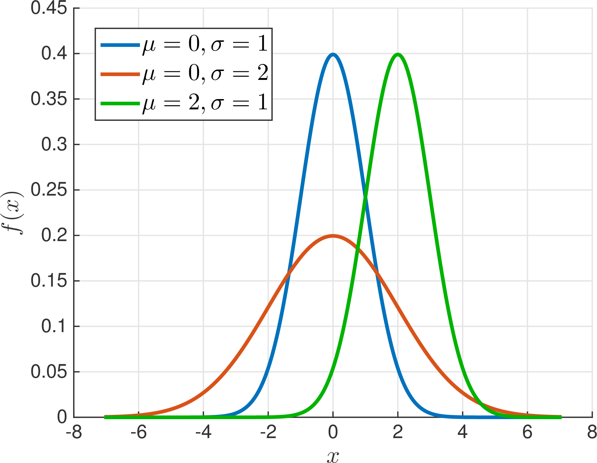
Figure 2: The density function for the normal distribution with several different choices for \(\mu\) and \(\sigma\).
The figure above shows that the normal density with different values of \(\mu\) and \(\sigma\) are very similar to each other. Indeed, the normal distribution has the following nice property with respect to shifting and rescaling.
Lemma 1
If \(X\) is a normal random variable with parameters \(\mu\) and \(\sigma\), then \(Y = (X - \mu)/\sigma\) is a standard normal random variable. Equivalently, if \(Y\) is a standard normal random variable, then \(X = \sigma Y + \mu\) has normal distribution with parameters \(\mu\) and \(\sigma\).
Proof. Given that \(X\) has normal distribution with parameters \(\mu\) and \(\sigma\), we can calculate the distribution of \(Y=(X - \mu)/\sigma\) as: \[{\mathbb{P}}[a\le Y\le b] = {\mathbb{P}}[\sigma a+\mu \le X\le \sigma b+\mu] = \frac{1}{\sqrt{2\pi\sigma^2}}\int_{\sigma a+\mu}^{\sigma b+\mu} e^{-(x-\mu)^2/(2\sigma^2)} \, {\mathrm{d}}x = \frac{1}{\sqrt{2\pi}}\int_{a}^{b} e^{-y^2/2} \, {\mathrm{d}}y,\] by a simple change of variable \(x = \sigma y + \mu\) in the integral. Hence \(Y\) is indeed standard normal. Note that \(Y\) is obtained from \(X\) just by shifting the origin to \(\mu\) and scaling by \(\sigma\). \(\square\)
Let us now calculate the expectation and variance of a normal random variable.
Theorem 3
For a normal random variable \(X\) with parameters \(\mu\) and \(\sigma\), \[{\mathbb{E}}[X] = \mu \qquad \text { and } \qquad {\operatorname{var}}(X) = \sigma^2.\]
Proof. Let’s first consider the case when \(X\) is standard normal, i.e., when \(\mu = 0\) and \(\sigma = 1\). By definition, its expectation is \[{\mathbb{E}}[X] = \int_{-\infty}^\infty xf(x) \, {\mathrm{d}}x = \frac{1}{\sqrt{2\pi}}\int_{-\infty}^\infty x e^{-x^2/2} \, {\mathrm{d}}x = \frac{1}{\sqrt{2\pi}}\left(\int_{-\infty}^0 x e^{-x^2/2} \, {\mathrm{d}}x +\int_{0}^\infty x e^{-x^2/2} \, {\mathrm{d}}x \right) = 0.\] The last step follows from the fact that the function \(e^{-x^2/2}\) is symmetrical about \(x=0\), so the two integrals are the same except for the sign. For the variance, we have \[\begin{aligned} {\operatorname{var}}(X) = {\mathbb{E}}[X^2] - {\mathbb{E}}[X]^2 &= \frac{1}{\sqrt{2\pi}}\int_{-\infty}^\infty x^2 e^{-x^2/2} \, {\mathrm{d}}x \\ &= \frac{1}{\sqrt{2\pi}}\bigl[-xe^{-x^2/2}\bigr]_{-\infty}^\infty + \frac{1}{\sqrt{2\pi}}\int_{-\infty}^\infty e^{-x^2/2} \, {\mathrm{d}}x \\ &=\frac{1}{\sqrt{2\pi}} \int_{-\infty}^\infty e^{-x^2/2} \, {\mathrm{d}}x = 1.\end{aligned}\] In the first line here we used the fact that \({\mathbb{E}}[X]=0\); in the second line we used integration by parts; and in the last line we used Equation 6 in the special case \(\mu=0\), \(\sigma=1\). So the standard normal distribution has expectation \({\mathbb{E}}[X]=0=\mu\) and variance \({\operatorname{var}}(X)=1=\sigma^2\).
Now consider the general case when \(X\) has normal distribution with general parameters \(\mu\) and \(\sigma\). By Lemma 1, we know that \(Y = (X - \mu)/\sigma\) is a standard normal random variable, so \({\mathbb{E}}[Y] = 0\) and \({\operatorname{var}}(Y) = 1\), as we have just established above. Therefore, we can read off the expectation and variance of \(X\) from those of \(Y\). For the expectation, using linearity, we have \[0 = {\mathbb{E}}[Y] = {\mathbb{E}}\!\left(\frac{X-\mu}{\sigma}\right) = \frac{{\mathbb{E}}[X]-\mu}{\sigma},\] and hence \({\mathbb{E}}[X] = \mu\). For the variance we have \[1 = {\operatorname{var}}(Y) = {\operatorname{var}}\!\left(\frac{X-\mu}{\sigma}\right) = \frac{{\operatorname{var}}(X)}{\sigma^2},\] and hence \({\operatorname{var}}(X)=\sigma^2\). \(\square\)
The bottom line, then, is that the normal distribution has expectation \(\mu\) and variance \(\sigma^2\). This explains the notation for the parameters \(\mu\) and \(\sigma\).
The fact that the variance is \(\sigma^2\) (so that the standard deviation is \(\sigma\)) explains our earlier comment that \(\sigma\) determines the “width” of the normal distribution. Namely, by Chebyshev’s inequality, a constant fraction of the distribution lies within distance (say) \(2\sigma\) of the expectation \(\mu\).
Note: The above analysis shows that, by means of a simple origin shift and scaling, we can relate any normal distribution to the standard normal. This means that, when doing computations with normal distributions, it’s enough to do them for the standard normal. For this reason, books and online sources of mathematical formulas usually contain tables describing the density of the standard normal. From this, one can read off the corresponding information for any normal r.v. \(X\) with parameters \(\mu,\sigma^2\), from the formula \[{\mathbb{P}}[X\le a] = {\mathbb{P}}\!\left[Y\le \frac{a-\mu}{\sigma}\right],\] where \(Y\) is standard normal.
The normal distribution is ubiquitous throughout the sciences and the social sciences, because it is the standard model for any aggregate data that results from a large number of independent observations of the same random variable (such as the heights of females in the US population, or the observational error in a physical experiment). Such data, as is well known, tends to cluster around its mean in a “bell-shaped" curve, with the correspondence becoming more accurate as the number of observations increases. A theoretical explanation of this phenomenon is the Central Limit Theorem, which we next discuss.
Sum of Independent Normal Random Variables
An important property of the normal distribution is that the sum of independent normal random variables is also normally distributed. We begin with the simple case when \(X\) and \(Y\) are independent standard normal random variables. In this case the result follows because the joint distribution of \(X\) and \(Y\) is rotationally symmetric. The general case follows from the translation and scaling property of normal distribution in Lemma 1.
Theorem 4
Let \(X\) and \(Y\) be independent standard normal random variables, and \(a,b \in \mathbb{R}\) be constants. Then \(Z = aX + bY\) is also a normal random variable with parameters \(\mu = 0\) and \(\sigma^2 = a^2 + b^2\).
Proof.3 Since \(X\) and \(Y\) are independent, by Theorem 1 we know that the joint density of \((X,Y)\) is \[f(x,y) = f(x) \cdot f(y) = \frac{1}{2\pi} e^{-(x^2+y^2)/2}.\] The key observation is that \(f(x,y)\) is rotationally symmetric around the origin, i.e., \(f(x,y)\) only depends on the value \(x^2 + y^2\), which is the distance of the point \((x,y)\) from the origin \((0,0)\); see Figure 3.
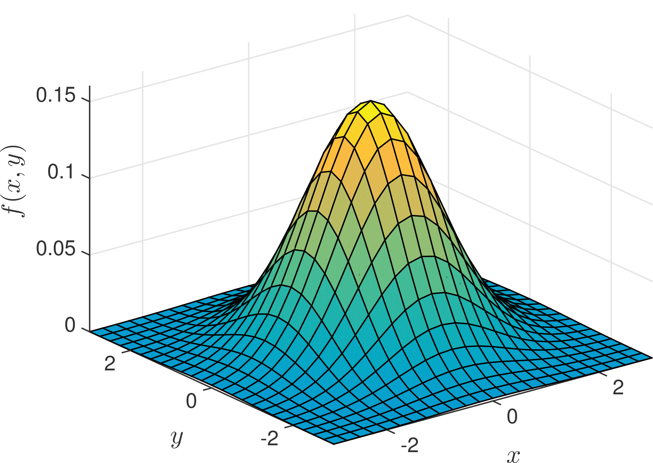
Figure 3: The joint density function \(f(x,y) = (2\pi)^{-1} e^{-(x^2+y^2)/2}\) is rotationally symmetric.
Thus, \(f(T(x,y)) = f(x,y)\) where \(T\) is any rotation of the plane \(\mathbb{R}^2\) about the origin. It follows that for any set \(A \subseteq \mathbb{R}^2\), \[ {\mathbb{P}}[(X,Y) \in A] = {\mathbb{P}}[(X,Y) \in T(A)]\](7) where \(T\) is a rotation of \(\mathbb{R}^2\). Now given any \(t \in \mathbb{R}\), we have \[{\mathbb{P}}[Z \le t] ~=~ {\mathbb{P}}[aX + bY \le t] ~=~ {\mathbb{P}}[(X,Y) \in A]\] where \(A\) is the half-plane \(\{(x,y) \mid ax + by \le t\}\). The boundary line \(ax+by = t\) lies at a distance \(d = t/\sqrt{a^2 + b^2}\) from the origin. Therefore, as illustrated in Figure 4, the set \(A\) can be rotated into the set \[T(A) = \left\{(x,y) : x \le \frac{t}{\sqrt{a^2+b^2}} \right\}.\]
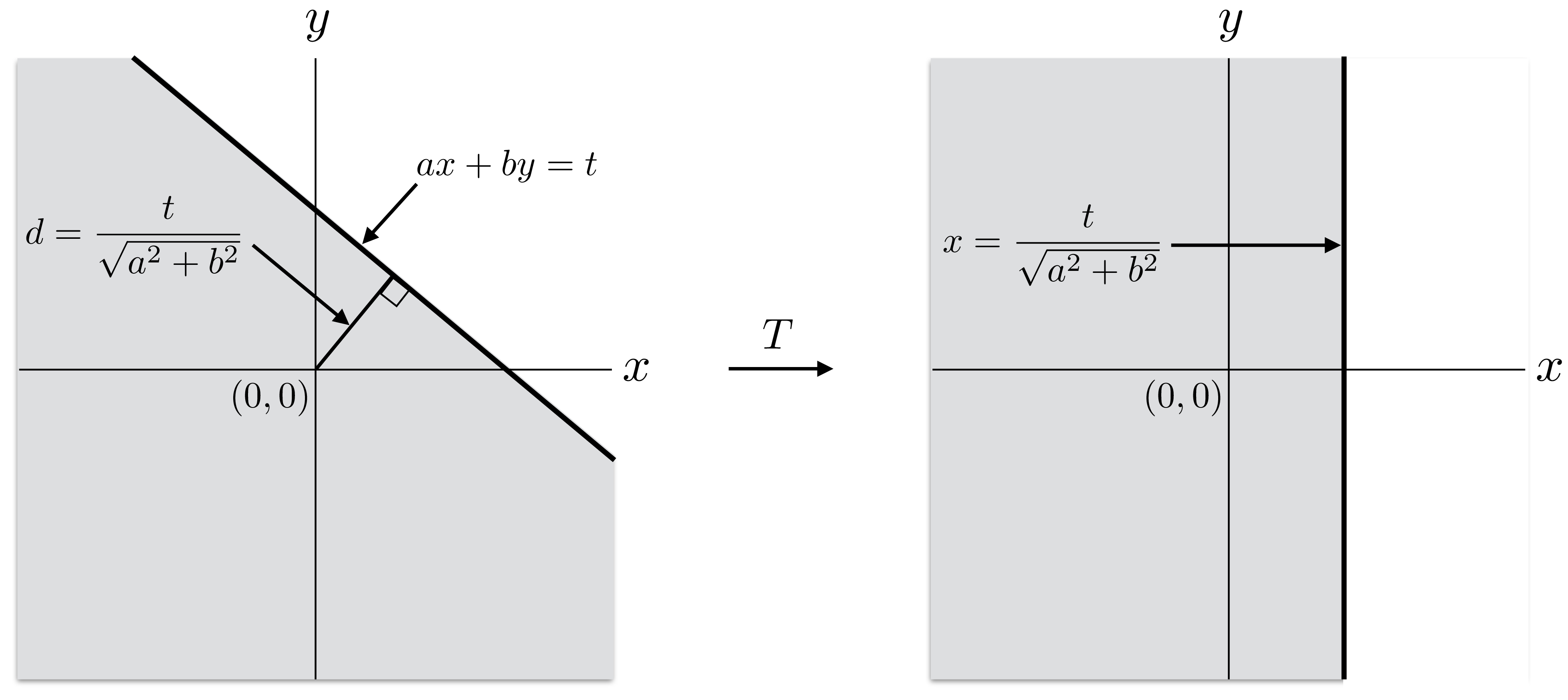
Figure 4: The half plane \(ax+by \le t\) is rotated into the half plane \(x \le t/\sqrt{a^2+b^2}\).
By Equation 7, this rotation does not change the probability: \[{\mathbb{P}}[Z \le t] ~=~ {\mathbb{P}}[(X,Y) \in A] ~=~ {\mathbb{P}}[(X,Y) \in T(A)] ~=~ {\mathbb{P}}\!\left[X \le \frac{t}{\sqrt{a^2+b^2}} \right] ~=~ {\mathbb{P}}\!\left[\sqrt{a^2+b^2} \, X \le t\right].\] Since the equation above holds for all \(t \in {\mathbb{R}}\), we conclude that \(Z\) has the same distribution as \(\sqrt{a^2+b^2} \, X\). Since \(X\) has standard normal distribution, we know by Lemma 1 that \(\sqrt{a^2 + b^2} \, X\) has normal distribution with mean \(0\) and variance \(a^2+b^2\). Hence we conclude that \(Z = aX + bY\) also has normal distribution with mean \(0\) and variance \(a^2+b^2\). \(\square\)
The general case now follows easily from Lemma 1 and Theorem 4.
Corollary 1
Let \(X\) and \(Y\) be independent normal random variables with parameters \((\mu_X, \sigma^2_X)\) and \((\mu_Y, \sigma^2_Y)\), respectively. Then for any constants \(a,b \in {\mathbb{R}}\), the random variable \(Z = aX + bY\) is also normally distributed with mean \(\mu = a\mu_X + b \mu_Y\) and variance \(\sigma^2 = a^2 \sigma_X^2 + b^2 \sigma_Y^2\).
Proof. By Lemma 1, \(Z_1 = (X - \mu_X) / \sigma_X\) and \(Z_2 = (Y - \mu_Y) / \sigma_Y\) are independent standard normal random variables. We can write: \[\begin{aligned} Z ~&=~ aX + bY ~=~ a(\mu_X + \sigma_X Z_1) + b(\mu_Y + \sigma_Y Z_2) ~=~ (a\mu_X + b\mu_Y) + (a\sigma_X Z_1 + b\sigma_Y Z_2).\end{aligned}\] By Theorem 4, \(Z' = a\sigma_X Z_1 + b\sigma_Y Z_2\) is normally distributed with mean \(0\) and variance \(\sigma^2 = a^2 \sigma_X^2 + b^2 \sigma_Y^2\). Since \(\mu = a\mu_X + b\mu_Y\) is a constant, by Lemma 1 we conclude that \(Z = \mu + Z'\) is a normal random variable with mean \(\mu\) and variance \(\sigma^2\), as desired. \(\square\)
The Central Limit Theorem
Recall from Note 18 the Law of Large Numbers for i.i.d. random variables \(X_i\)’s: it says that the probability of any deviation \(\alpha\) of the sample average \(A_n := n^{-1} {\sum_{i=1}^n X_i}\) from the mean, however small, tends to zero as the number of observations \(n\) in our average tends to infinity. Thus by taking \(n\) large enough, we can make the probability of any given deviation as small as we like.
Actually we can say something much stronger than the Law of Large Numbers: namely, the distribution of the sample average \(A_n\), for large enough \(n\), looks like a normal distribution with mean \(\mu\) and variance \(\sigma^2/n\). (Of course, we already know that these are the mean and variance of \(A_n\); the point is that the distribution becomes normal!) The fact that the standard deviation decreases with \(n\) (specifically, as \(\sigma/\sqrt{n}\)) means that the distribution approaches a sharp spike at \(\mu\).
Recall from the last section that the density of the normal distribution is a symmetrical bell-shaped curve centered around the mean \(\mu\). Its height and width are determined by the standard deviation \(\sigma\) as follows: the height at the mean \(x = \mu\) is \(1/\sqrt{2\pi \sigma^2} \approx 0.4/\sigma\); \(50\%\) of the mass is contained in the interval of width \(0.67\sigma\) either side of the mean, and \(99.7\%\) in the interval of width \(3\sigma\) either side of the mean. (Note that, to get the correct scale, deviations are on the order of \(\sigma\) rather than \(\sigma^2\).)
To state the Central Limit Theorem precisely (so that the limiting distribution is a constant rather than something that depends on \(n\)), we shift the mean of \(A_n\) to \(0\) and scale it so that its variance is \(1\), i.e., we replace \(A_n\) by \[A'_n = \frac{(A_n-\mu)\sqrt{n}}{\sigma} = \frac{\sum_{i=1}^n X_i -n\mu}{\sigma\sqrt{n}}.\] The Central Limit Theorem then says that the distribution of \(A'_n\) converges to the standard normal distribution.
Theorem 5
Let \(X_1,X_2,\ldots,X_n\) be i.i.d. random variables with common expectation \(\mu={\mathbb{E}}[X_i]\) and variance \(\sigma^2={\operatorname{var}}(X_i)\) (both assumed to be \(<\infty\)). Define \(A'_n = (\sum_{i=1}^n X_i -n\mu)/(\sigma\sqrt{n})\). Then as \(n\to\infty\), the distribution of \(A'_n\) approaches the standard normal distribution in the sense that, for any real \(\alpha\), \[{\mathbb{P}}[A'_n \le \alpha] \to \frac{1}{\sqrt{2\pi}}\int_{-\infty}^\alpha e^{-x^2/2} \, {\mathrm{d}}x\quad\text{as $n\to\infty$}.\]
The Central Limit Theorem is a very striking fact. What it says is the following: If we take an average of \(n\) observations of any arbitrary r.v. \(X\), then the distribution of that average will be a bell-shaped curve centered at \(\mu={\mathbb{E}}[X]\). Thus all trace of the distribution of \(X\) disappears as \(n\) gets large: all distributions, no matter how complex,4 look like the normal distribution when they are averaged. The only effect of the original distribution is through the variance \(\sigma^2\), which determines the width of the curve for a given value of \(n\), and hence the rate at which the curve shrinks to a spike.
Optional: Buffon’s Needle
Here is a simple yet interesting application of continuous random variables to the analysis of a classical procedure for estimating the value of \(\pi\) known as Buffon’s needle, after its 18th century inventor Georges-Louis Leclerc, Comte de Buffon.
Here we are given a needle of length \(\ell\), and a board ruled with horizontal lines at distance \(\ell\) apart. The experiment consists of throwing the needle randomly onto the board and observing whether or not it crosses one of the lines. We shall see below that (assuming a perfectly random throw) the probability of this event is exactly \(2/\pi\). This means that, if we perform the experiment many times and record the proportion of throws on which the needle crosses a line, then the Law of Large Numbers tells us that we will get a good estimate of the quantity \(2/\pi\), and therefore also of \(\pi\); and we can use Chebyshev’s inequality as in the other estimation problems we considered in that same Note to determine how many throws we need in order to achieve specified accuracy and confidence.
To analyze the experiment, let’s consider what random variables are in play. Note that the position where the needle lands is completely specified by two random variables: the vertical distance \(Y\) between the midpoint of the needle and the closest horizontal line, and the angle \(\Theta\) between the needle and the vertical. The r.v. \(Y\) ranges between \(0\) and \(\ell/2\), while \(\Theta\) ranges between \(-\pi/2\) and \(\pi/2\). Since we assume a perfectly random throw, we may assume that their joint distribution has density \(f(y,\theta)\) that is uniform over the rectangle \([0,\ell/2]\times[-\pi/2,\pi/2]\). Since this rectangle has area \(\pi \ell/2\), the density should be \[ f(y,\theta) = \begin{cases} 2/\pi\ell & \text{for $(y,\theta)\in [0,\ell/2]\times[-\pi/2,\pi/2]$;}\cr 0 & \text{otherwise}.\cr \end{cases}\](8) Equivalently, \(Y\) and \(\Theta\) are independent random variables, each uniformly distributed in their respective range. As a sanity check, let’s verify that the integral of this density over all possible values is indeed \(1\): \[\int_{-\infty}^\infty \int_{-\infty}^\infty f(y,\theta) \, {\mathrm{d}}y \, {\mathrm{d}}\theta = \int_{-\pi/2}^{\pi/2}\int_0^{\ell/2} \frac{2}{\pi\ell} \, {\mathrm{d}}y \, {\mathrm{d}}\theta = \int_{-\pi/2}^{\pi/2} \left[\frac{2y}{\pi\ell}\right]_0^{\ell/2} \, {\mathrm{d}}\theta = \int_{-\pi/2}^{\pi/2} \frac{1}{\pi} \, {\mathrm{d}}\theta = \left[\frac{\theta}{\pi}\right]_{-\pi/2}^{\pi/2} = 1.\] This is an analog of Equation 1 for our joint distribution; rather than the area under the curve \(f(x)\), we are now computing the area under the “surface" \(f(y,\theta)\).
Now let \(E\) denote the event that the needle crosses a line. How can we express this event in terms of the values of \(Y\) and \(\Theta\)? Well, by elementary geometry the vertical distance of the endpoint of the needle from its midpoint is \((\ell/2)\cos\Theta\), so the needle will cross the line if and only if \(Y\le (\ell/2)\cos\Theta\). Therefore we have \[{\mathbb{P}}[E] = {\mathbb{P}}\!\left[Y \le \frac{\ell}{2}\cos\Theta\right] = \int_{-\pi/2}^{\pi/2}\int_0^{(\ell/2)\cos\theta} f(y,\theta)\, {\mathrm{d}}y \, {\mathrm{d}}\theta.\]
Substituting the density \(f(y,\theta)\) from Equation 8 and performing the integration we get \[{\mathbb{P}}[E] = \int_{-\pi/2}^{\pi/2}\int_0^{(\ell/2)\cos\theta} \frac{2}{\pi\ell} \, {\mathrm{d}}y \, {\mathrm{d}}\theta = \int_{-\pi/2}^{\pi/2} \left[\frac{2y}{\pi\ell}\right]_0^{(\ell/2)\cos\theta} \, {\mathrm{d}}\theta = \frac{1}{\pi}\int_{-\pi/2}^{\pi/2} \cos\theta \, {\mathrm{d}}\theta = \frac{1}{\pi}\left[\sin\theta\right]_{-\pi/2}^{\pi/2} = \frac{2}{\pi}.\]
This is exactly what we claimed at the beginning of the section!
Buffon’s Needle: A Slick Approach
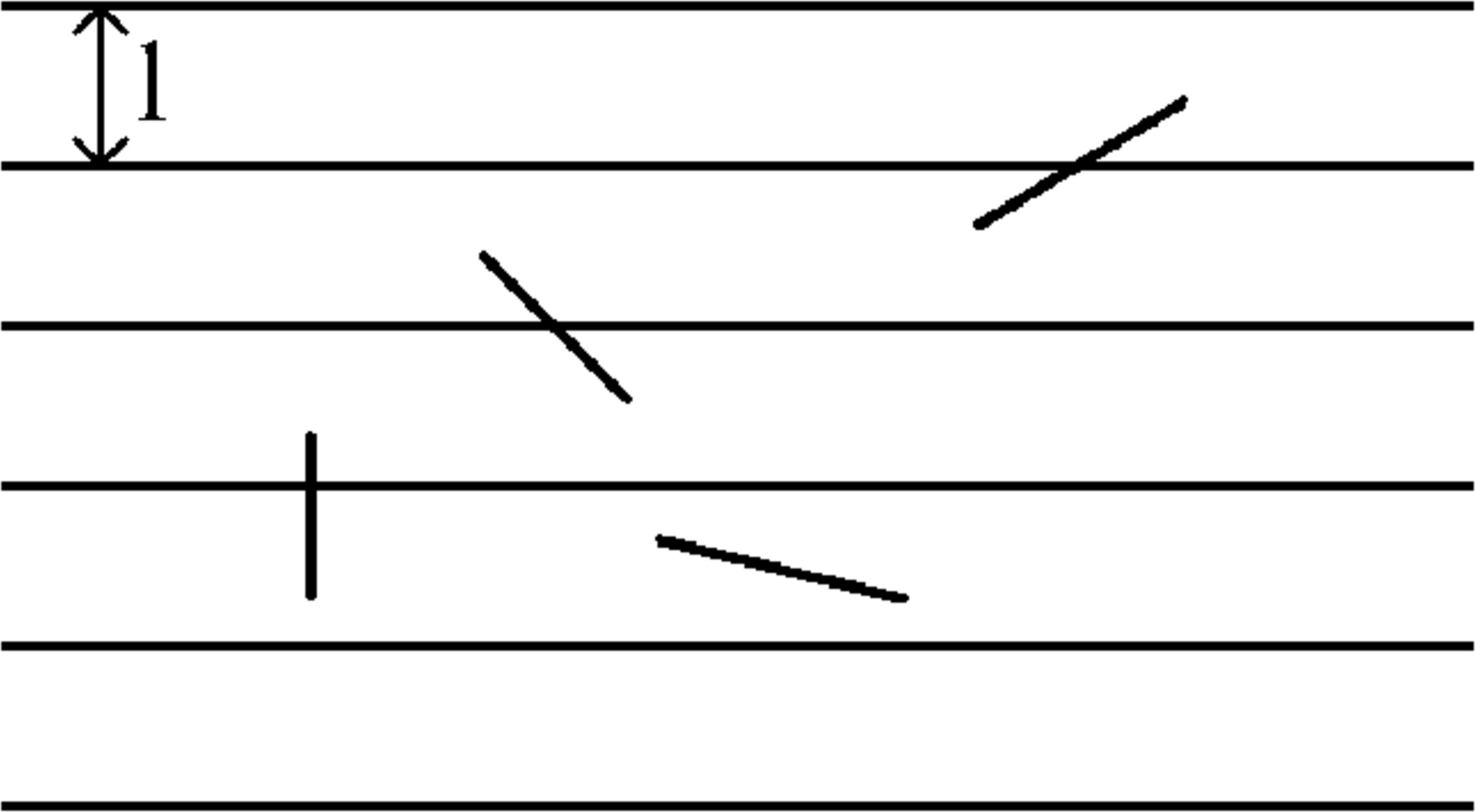
Figure 5: Buffon’s Needle.
Recall that we toss a unit length needle on (an infinite) board ruled with horizontal lines spaced at unit length apart. We wish to calculate the chance that the needle intersects a horizontal line. That is, let \(I\) be the event that the needle intersects a line. We will show that \({\mathbb{P}}[I] = 2/\pi\). Let \(X\) be a random variable defined to be the number of intersections of such a needle: \[X = \left\{ \begin{array}{cc} 1&\mbox{ if the needle intersects a line }\\ 0&\mbox{ otherwise. } \end{array}\right.\]
Since \(X\) is an indicator random variable, \({\mathbb{E}}[X] = {\mathbb{P}}[I]\) (here we are assuming the case in which the needle lies perfectly on two lines cannot happen, since the probability of this particular event is \(0\)). Now, imagine that we were tossing a needle of two unit length, and we let \(Z\) be the random variable representing the number of times such a needle intersects horizontal lines on the plane. We can “split" the needle into two parts of unit length and get \(Z = X_1 + X_2\), where \(X_i\) is \(1\) if segment \(i\) of the needle intersects and \(0\) otherwise. Thus, \({\mathbb{E}}[Z] = {\mathbb{E}}[X_1 + X_2] = {\mathbb{E}}[X_1] + {\mathbb{E}}[X_2] = 2{\mathbb{E}}[X]\), since each segment is of unit length. A similar argument holds if we split a unit length needle into \(m\) equal segments, so that \(X = X_1 + \cdots + X_m\), where \(X_i\) is \(1\) if segment \(i\) (which has length \(1/m\)) intersects a line and \(0\) otherwise. We have that \({\mathbb{E}}[X] = {\mathbb{E}}[X_1 + \cdots + X_m] = {\mathbb{E}}[X_1] + \cdots + {\mathbb{E}}[X_m]\). But each of the \({\mathbb{E}}[X_i]\)s are equal, so we get \({\mathbb{E}}[X] = m{\mathbb{E}}[X_i] \rightarrow {\mathbb{E}}[X_i] = (\text{length of segment $i$}) \cdot {\mathbb{E}}[X]\). Thus, if we drop a needle of length \(l\), and we let \(Y\) be the number of intersections, then \({\mathbb{E}}[Y] = l \cdot {\mathbb{E}}[X]\). Even if we have a needle which is arbitrarily short, say length \(\epsilon\), we still have \({\mathbb{E}}[Y] = \epsilon \cdot {\mathbb{E}}[X]\).
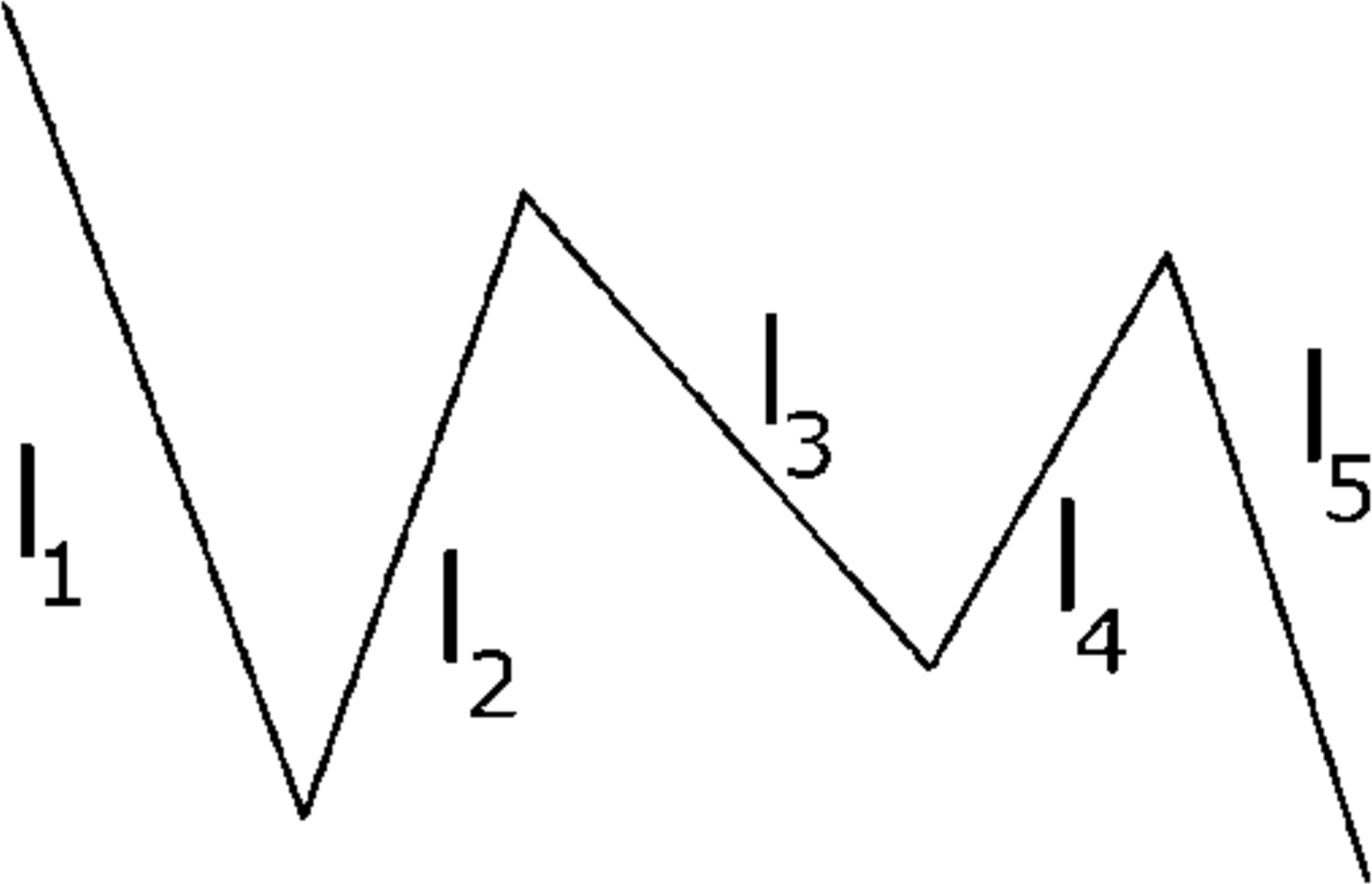
Figure 6: “Noodle” consisting of \(5\) needles.
Now, consider a “noodle" comprised of two needles of arbitrary lengths \(l_1\) and \(l_2\) (with corresponding random variables \(X_1\) and \(X_2\)), where the needles are connected by a rotating joint, we can conclude by linearity of expectation that \({\mathbb{E}}[X_1 + X_2] = {\mathbb{E}}[X_1] + {\mathbb{E}}[X_2]\). In general, we can have a noodle comprised of \(n\) needles of arbitrary length: where \({\mathbb{E}}[X_1 + \cdots + X_n] = {\mathbb{E}}[X_1] + \cdots + {\mathbb{E}}[X_n] = l_1{\mathbb{E}}[X] + \cdots + l_n{\mathbb{E}}[X]\). Factoring \({\mathbb{E}}[X]\) out, we get that the expected number of intersections of a noodle is \((\text{length of noodle}) \cdot {\mathbb{E}}[X]\). In particular, since we are allowed to string together needles at connected rotating joints and since each needle can be arbitrarily short, we are free to pick any shape, but which one?
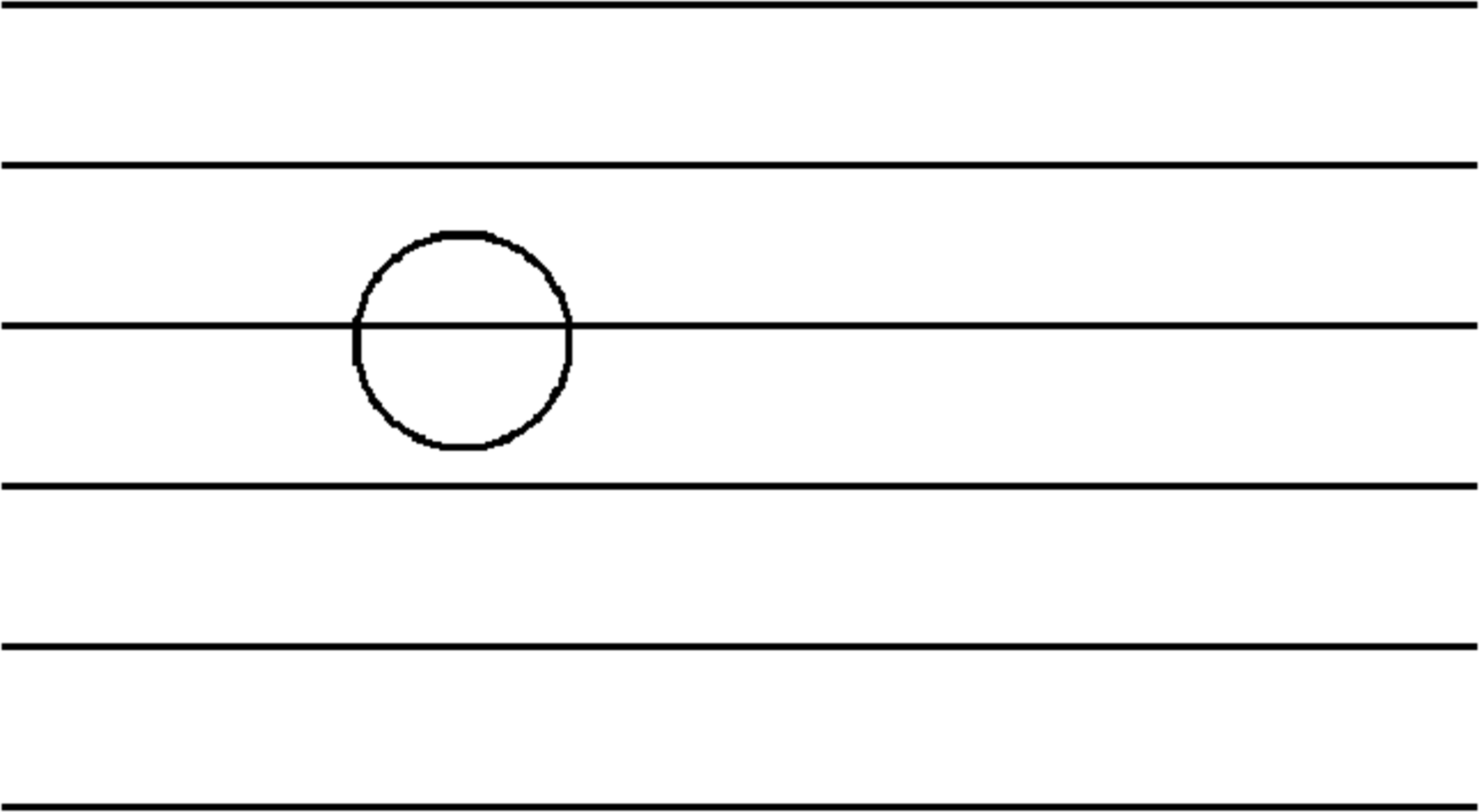
Figure 7: A circle always has two intersections.
Consider a circle with a unit length diameter (and therefore circumference \(\pi\)). Such a shape must always intersect twice: which implies \({\mathbb{E}}[\text{number of circle intersections}] = \pi \cdot {\mathbb{E}}[X] = 2\), and thus \({\mathbb{E}}[X] = 2/\pi = {\mathbb{P}}[I]\).
A formal treatment of which events can be assigned a well-defined probability requires a discussion of measure theory, which is beyond the scope of this course.↩
Note that it does not matter whether or not we include the endpoints \(a,b\); since \({\mathbb{P}}[X=a]={\mathbb{P}}[X=b]=0\), we have \({\mathbb{P}}[a< X< b] = {\mathbb{P}}[a\le X\le b]\).↩
The following proof and figures are adapted from “Why Is the Sum of Independent Normal Random Variables Normal?” by B. Eisenberg and R. Sullivan, Mathematics Magazine, Vol. 81, No. 5.↩
We do need to assume that the mean and variance of \(X\) are finite.↩